Working Set Reduction - Design Document

Working set reduction decomposes operations or sequences of operations into loops doing computations in a piecewise manner, for instance decomposing a large matrix multiplication x @ y into a series of multiplications on groups of x’s rows. The resulting operations operate on smaller tensors with the following benefits:

• Smaller tensors help alleviate hardware limitations with respect to per-core, per-tensor DDR/HBM access span.

• Smaller tensors help reduce memory bandwidth pressure by making it possible to keep tensors in scratchpad memory.

This document motivates and walks through the working set reduction approach adopted in torch-spyre.

Quick navigation:

• Approach

• Working set reduction hints

• Example 1: naming dimensions and tiling

• Dimensions vs. named dimensions

• Example 2: view-based dimension splitting

• Implementation

  • Intermediate representation

  • Lowering

  • Transformation

• Related documents

Approach

We intend to support both implicit (compiler generated) and explicit (source code driven) working set reduction. In the short term, the latter makes it possible to decouple the effort on working set reduction heuristics from downstream tasks (intermediate representations, analyses, and transformations). Eventually, the combination of the two can result in better performance and productivity than either solution in isolation.

Explicit working set reduction can be decomposed in four stages:

1. Introduce source-level hints on operations and tensors to drive working set reduction.

2. Introduce encodings of working set reduction decisions as metadata on LLIR operations and buffers.

3. Lower source-level hints to IR metadata.

4. Transform the annotated IR into an executable program.

Implicit working set reduction via compiler heuristics reuses stage 2 and beyond.

The classic illustration is a matrix multiplication. Given z = x @ y with x: [M, K] and y: [K, N], multiple tiling choices are valid: tile x along M, tile y along N, tile both, or tile the reduction axis K. Tiling along non-reduction axes produces independent output tiles. Tiling along the reduction axis is qualitatively different: each tile produces a partial sum, and an extra accumulation step combines them.

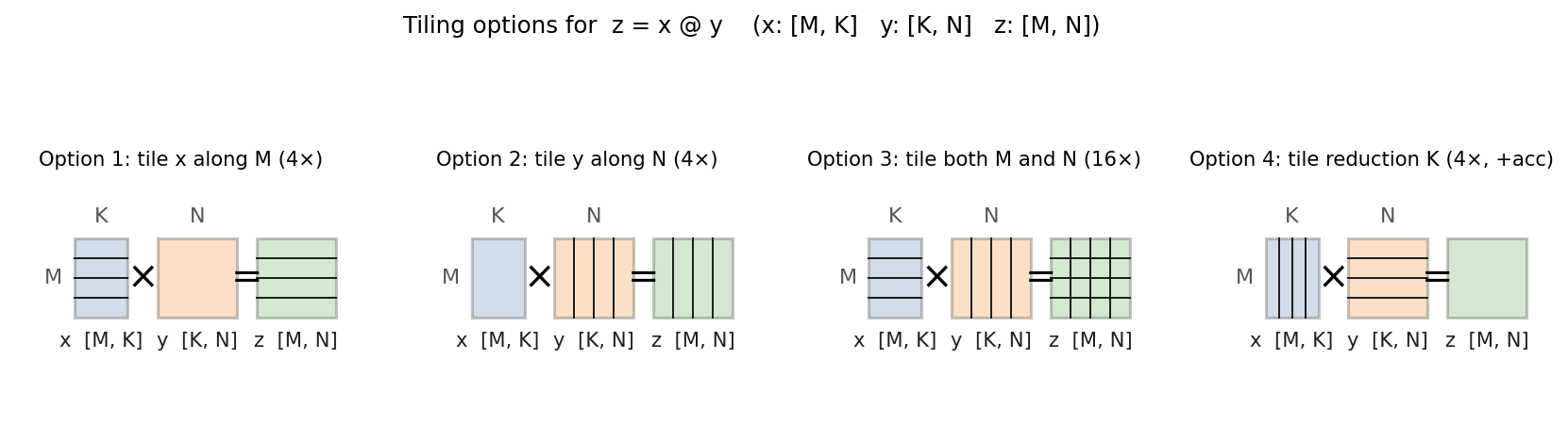
Tiling options for a matrix multiplication. Options 1-3 tile non-reduction axes; each tile is independent. Option 4 tiles the reduction axis K and introduces an extra accumulation step.

Working set reduction hints

To explicitly control working set reduction, we name tensor dimensions and tile them.

Example 1: Naming Dimensions and Tiling

M, K, N = 64, 256, 128

declare_tensor_dim("M", M)
declare_tensor_dim("K", K)
declare_tensor_dim("N", N)


def kernel(x, y, z):
    with spyre_hint(tiles={"M": 8}):
        with spyre_hint(tiles={"K": 4}):
            p = x @ y
        return p + z


x = torch.rand(M, K, dtype=torch.float16).to("spyre")
y = torch.rand(K, N, dtype=torch.float16).to("spyre")
z = torch.rand(M, N, dtype=torch.float16).to("spyre")

name_tensor_dims(x, ["M", "K"])
name_tensor_dims(y, ["K", "N"])
name_tensor_dims(z, ["M", "N"])

print(torch.compile(kernel)(x, y, z))

In this example, we declare three tensor dimensions "M", "K", and "N" using declare_tensor_dim, map three device tensors to these dimensions using name_tensor_dims and finally tile the "M" and "K" dimensions using spyre_hint. The matmul operation is tiled along both "M" and "K" whereas the final add operation is only tiled along "M".

Hints are introduced with the with spyre_hint(**kwargs): pattern. Working set reduction hints utilize the tiles keyword and consist of a dictionary mapping dimension names to per-dimension tile counts. The value is the number of tiles to split that dimension into: tiles={"M": 8} produces 8 tiles along M, each of size M/8.

Multiple dimensions can be tiled at once. Since "K" does not occur in tensor z or p, the example code is equivalent to:

def kernel(x, y, z):
    with spyre_hint(tiles={"M": 8, "K": 4}):
        return x @ y + z

Named tensor dimensions must be provided for inputs to torch.compile but are intended to be derived most of the time for computed tensors.

Dimensions vs. named dimensions

Named dimensions are deliberately distinct from tensor shape:

Dimensions are ephemeral and reflect the current view. Named dimensions are durable and reflect the intent and storage.

A 2D tensor and its flatten() produce different tensor.shape values but keep the same named dimensions. Two flat 1D tensors with reversed naming order are not equivalent even though their shapes match.

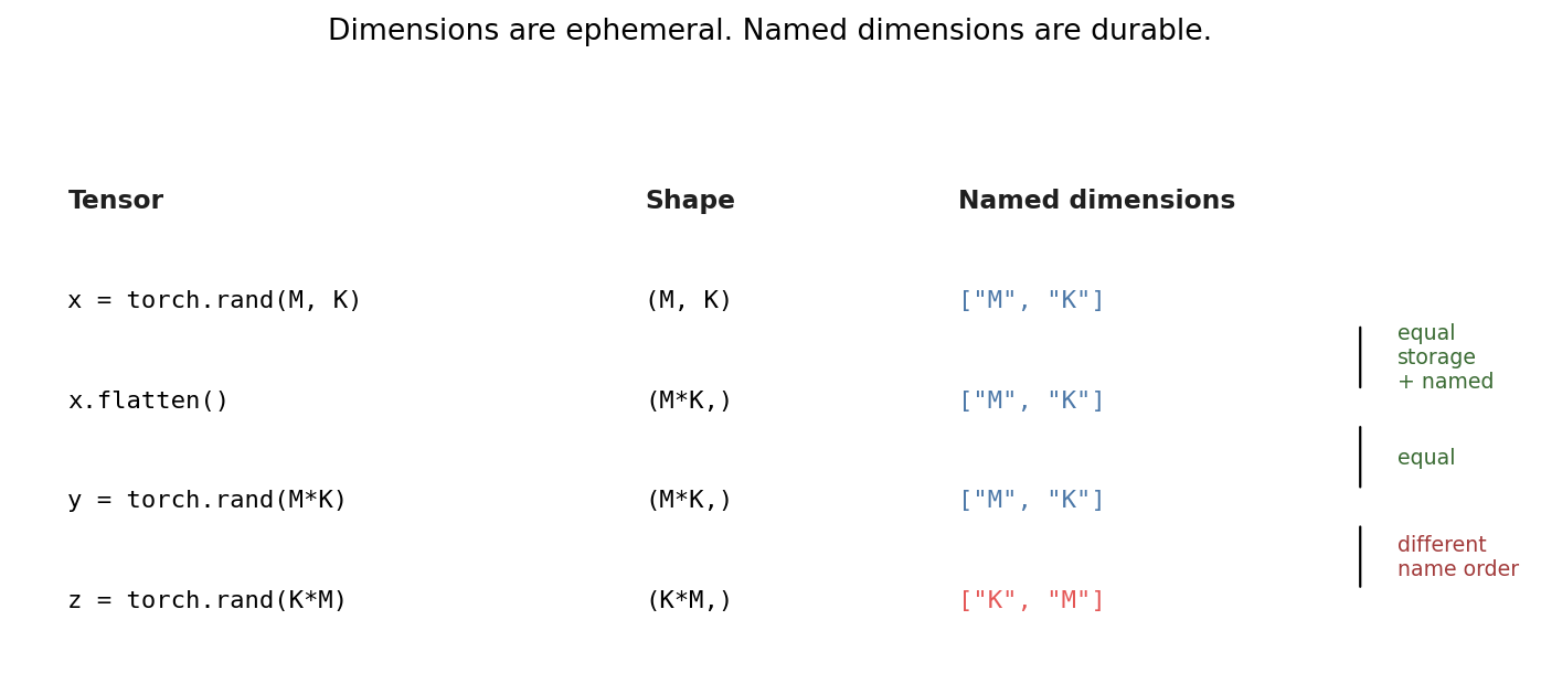
Named dimensions track the intent of the tensor’s storage and survive view transformations like flatten(). Reversed name order produces a tensor that is not equivalent even when the shape matches.

This separation is what allows hints to refer to logical axes ("M", "K", "N") regardless of whether intermediate views have collapsed or re-shaped them.

Example 2: View-Based Dimension Splitting

Named tensor dimensions are intended to reflect the tensor layout in memory. For instance, the following code is valid:

def kernel(x_1d, y, z):
    with spyre_hint(tiles={"M": 8, "K": 4}):
        return x_1d.view(M, K) @ y + z

x_1d = torch.rand(M * K, dtype=torch.float16).to("spyre")

name_tensor_dims(x_1d, ["M", "K"])

Here the name_tensor_dims invocation records that x_1d while declared as a 1d tensor is in essence a 2d tensor with outer dimension "M" and inner dimension "K". Consequently, the count of dimensions of a tensor or view may be different from its named dimension count.

The order of named dimensions is significant. The following two declarations are not equivalent:

name_tensor_dims(x, ["M", "K"]) # M before K
name_tensor_dims(x, ["K", "M"]) # K before M

Named tensor dimensions are expected to be consistent with the mathematical properties of the operations involving the tensors. For instance, in x @ y there must exist n>0 such that x_named_dims[-n:] == y_named_dims[:n], as for instance with named dimensions ["A", "B", "C", "D"] for x and ["C", "D", "E"] for y. In this example, the reduction dimension is the flattened dimension ["C", "D"].

Implementation

Intermediate representation

Hints are automatically assigned a unique id.

We extend LLIR as follows:

• We add a list of computed dimensions to each computed buffer.

• We add iteration dimensions to each operation mapping iteration variables to lists of named dimensions.

• We add hints to each operation mapping hint ids to the hint values for every enclosing hint.

For instance, for x @ y in our example, we add:

• Computed dimensions: ["M", "N"]

• Iteration dimensions: {d0: ["M"], d1: ["K"], d2: ["N"]} assuming variables d0, d1, and d2 respectively map to dim 0 of x, the reduction dimension, and dim 1 of y.

• Hints: {3: {"tiles": {"M": 8}}, 4: {"tiles": {"K": 4}}}

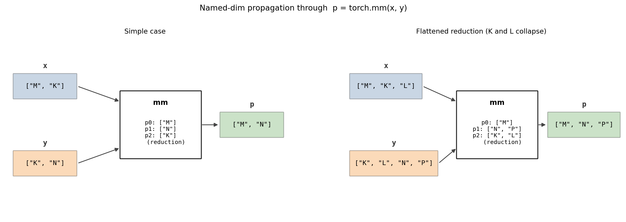
Named dimensions on the inputs determine the iteration-variable mapping on the operation, which in turn determines the named dimensions of the output. The right-hand panel illustrates the flattened-reduction case where two input dimensions collapse into a single iteration variable.

Hint ids are positive integers. They are unique, not in general consecutive, but they respect the nesting order. Concretely, if a hint is nested inside another hint, the inner hint id will be greater than the outer hint id.

Hint ids make it possible to reconstruct hint scopes from operation metadata. Nested with spyre_hint(...) blocks form a tree that can be recovered from the recorded ids.

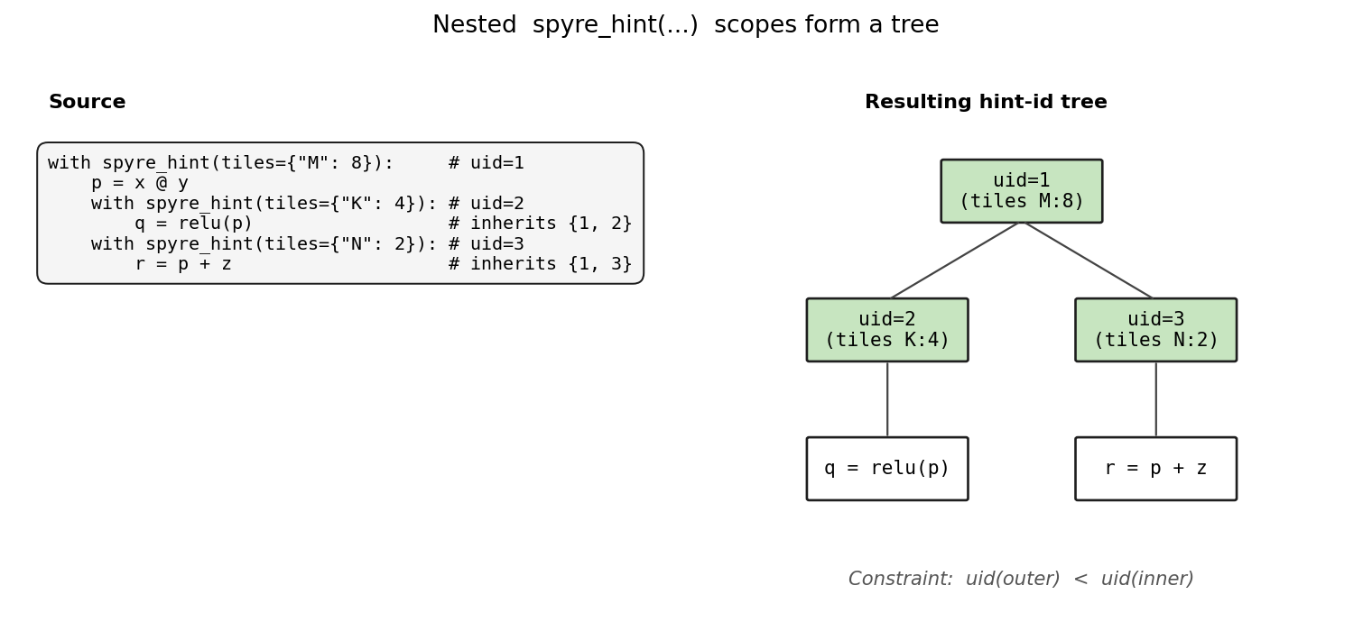
Each spyre_hint(...) block gets a unique, monotonically increasing id. Operations inherit every enclosing hint, and the partial order on ids recovers the nesting tree.

Lowering

Spyre hints are captured on the FX graph using the torch.fx.traceback.annotate context manager and preserved through AOT using custom pre- and post-AOT passes to save and restore the hints. Node matching pre- and post-AOT relies on topological sorting.

Hints on LLIR operations are derived from origin FX nodes on demand via a getter method (get_op_hints).

Named tensor dimensions are specified only on input tensors. To use these names for optimization throughout the PyTorch graph, they must be propagated to intermediate tensors produced by operations. This requires propagating dimension name metadata through the Inductor intermediate representation. This is implemented by the propagate_named_dims pass.

In most cases, tracking dimension names through operations is straightforward. The primary complexity comes from handling views, particularly views that split or combine dimensions, as shown in Example 2.

The current implementation assumes that when a view splits a dimension, the input tensor’s corresponding dimension already contains the necessary number of dimension names with compatible sizes (for example, ["M", "K"] in Example 2). Named dimensions are propagated through intermediate tensors and aligned to tensor dimensions using stride-based analysis, ensuring correctness under view transformations.

More automated dimension naming is planned. In the current implementation, if an input dimension is unnamed, or if a view transformation is inconsistent with the user-provided dimension names, a warning is emitted and propagation continues with partial or inferred information.

The pass runs in CustomPreSchedulingPasses, after tensor layouts have been finalized and before work-division and scratchpad planning consume the resulting iteration spaces. The slot is rigid: layouts must be settled before tiling decisions can refer to them, and work-division must see the post-tiling iteration space.

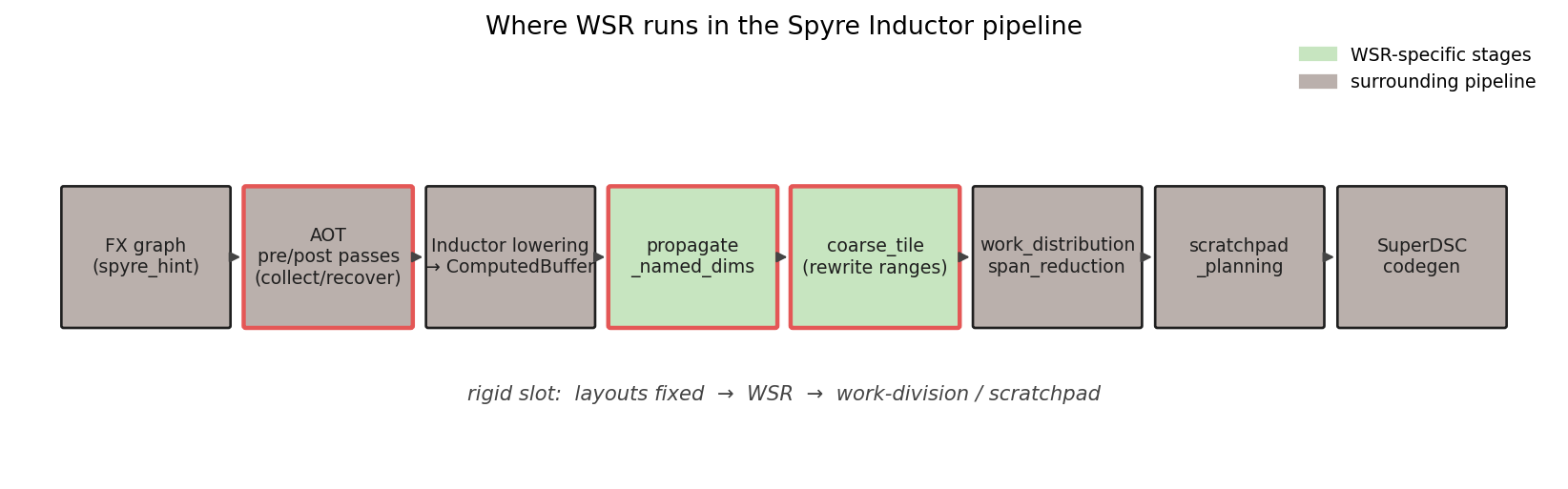
WSR-specific stages (highlighted) sit between Inductor lowering and work-division/scratchpad planning. AOT pre/post passes preserve hint metadata across retracing.

Transformation

The annotated IR is transformed into a tiled loop nest by the coarse-tiling pass. Each contiguous run of operations sharing the same tiling decision is rewritten with reduced per-iteration ranges, wrapped in a counted loop, and emitted as nested LoopSpec structures that the SuperDSC codegen lowers to hardware MLIR (scf.for + affine.apply + sdsc_execute).

The reduction in working set is what makes intermediates fit in LX scratchpad: an intermediate buffer that is produced and consumed inside the same loop iteration never needs an HBM allocation.

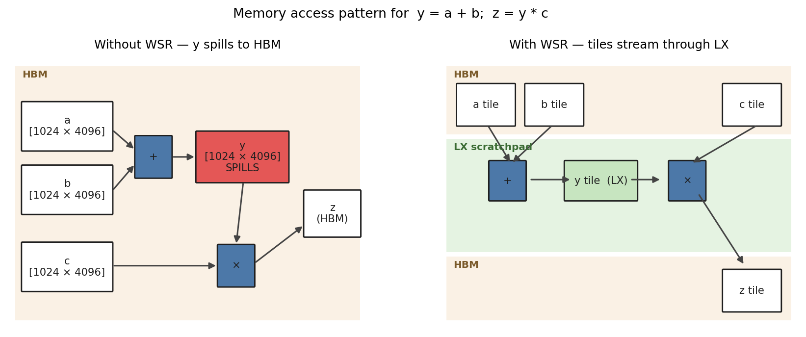
For y = a + b; z = y * c: without WSR, the intermediate y is full-size and spills to HBM. With WSR, each tile of y lives in LX scratchpad for the duration of one iteration and is consumed immediately by the next op.

The full mechanics — how loop identity is carried through Inductor’s flat-list pipeline, how the loop perimeter prevents cross-group fusion, how buffers crossing the loop boundary are classified — are documented in coarse_tiling_loops.md. The design rationale for those mechanics is in RFC #16: Coarse Tiling.

Related documents

• coarse_tiling_loops.md — implementation reference for the transformation stage (Layer 1 IR pass, Layer 2 scheduler wrapper, Layer 3 codegen tree).

• RFC #16: Coarse-Tiling Loop IR — Design Rationale — why the three-layer design has the shape it does.

• scratchpad_planning.md — how LX scratchpad allocation consumes the per-tile iteration spaces produced by WSR.

• work_division_planning.md — how work distribution across cores runs after WSR on the reduced ranges.